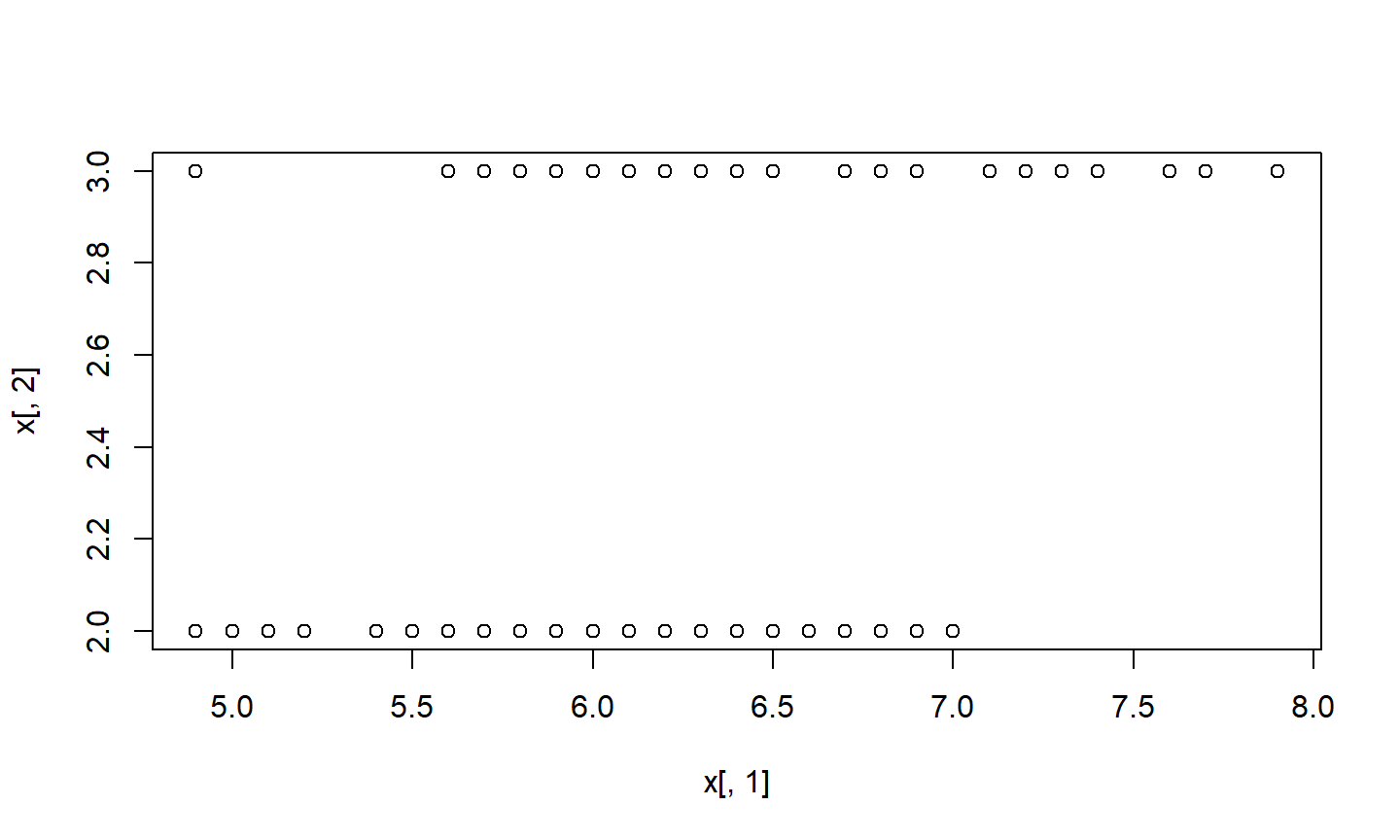
Feb., 2021

Iris data set

Iris data set

plot(x[,1],x[,2]) #plot of Species vs. sepal lengths

Serial mode

we will use the foreach function from the doParallel package to fit the data to a generalized linear model.

library(doParallel)

Serial mode

Let’s take a look at the performance of a logistic regression model in serial mode (1 core):

stime <- system.time({
    r <- foreach(1:10000, .combine=cbind) %do% {
        train <- sample(100,100, replace=TRUE)
        result1 <- glm(x[train,2]~x[train,1], family=binomial(logit))
        coefficients(result1)
    }
})[3]
stime
## elapsed 
##   22.24

Parallel mode

Now, look at the performance using 2 cores:

cl <- makeCluster(2)
registerDoParallel(cl)
ptime <- system.time({
    r <- foreach(1:10000, .combine=cbind) %dopar% {
        train <- sample(100,100, replace=TRUE)
        result1 <- glm(x[train,2]~x[train,1], family=binomial(logit))
        coefficients(result1)
    }
})[3]
ptime
## elapsed 
##   16.11
stopCluster(cl)

Parallel mode

a graphical view of the scaling behavior can be seen in the following plot:

Is parallel processing always the best alternative?

stime <- system.time(
        foreach(i=1:1e4) %do% sqrt(i) )
stime 
##    user  system elapsed 
##    1.73    0.00    1.73
cl <- makeCluster(2)
registerDoParallel(cl)
ptime <- system.time( 
        foreach(i=1:1e4) %dopar% sqrt(i) )
ptime 
##    user  system elapsed 
##    2.65    0.26    3.24
stopCluster(cl)

Is parallel processing always the best alternative?

Only if the computational load (number of numerical operations) exceeds the overhead of using the parallel routines.

Another message from these examples is that one always needs to check the performance of the code (Time) vs. the number of requested cores, to use an “optimal” number.

These data can be useful upon applying for medium/large SNIC projects because the reviewers would know if the requested hours are justified.

References