There are some tricks you can follow in order to get a faster code, we will use our Pi function from the previous topic as our baseline:

sim <- function(l) {
  c <- rep(0,l); hits <- 0
  pow2 <- function(x) { x2 <- sqrt( x[1]*x[1]+x[2]*x[2] ); return(x2) }
  for(i in 1:l){
             x = runif(2,-1,1)
     if( pow2(x) <=1 ){
                  hits <- hits + 1
        }
        dens <- hits/i; pi_partial = dens*4; c[i] = pi_partial
    }
   return(c)
}

the execution time of this function for 100,000 iterations is

size <- 100000
system.time(
   res <- sim(size)
)

##    user  system elapsed 
##     0.6     0.0     0.8

If we vectorize the code we obtain a better performance:

simv <- function(l) {
  set.seed(0.234234)
  x=runif(l); y=runif(l)
  z=sqrt(x^2 + y^2)
  resl <- length(which(z<=1))*4/length(z)
  return(resl)
}

size <- 100000
system.time(
  res <- simv(size)
)

##    user  system elapsed 
##    0.01    0.00    0.02

a message from this example is that loops are expensive in R and vectorization can help to improve the performance of the code.

Common vector operations: \(+\), \(-\), \(/\), \(*\), \(\% * \%\).

N <- 1E5
data1 <- 1 
system.time({
    for (j in 2:N) {
      data1 <- c(data1, data1[j-1] + sample(-5:5, size=1))
    }
  })

##    user  system elapsed 
##   11.83    0.02   12.52

data2 <- numeric(N)
data2[1] <- 1
system.time({
  for (j in 2:N) {
    data2[j] <- data2[j-1] + sample(-5:5, size=1)
  }
})

##    user  system elapsed 
##    0.58    0.00    0.58

This example shows that pre-allocating memory reduces the execution time.

data1 <- rnorm(1E4*1000)
dim(data1) <- c(1E4,1000)
dataf <- data.frame(data1)
system.time(data2 <- rowSums(dataf))

##    user  system elapsed 
##    0.05    0.00    0.05

data1 <- rnorm(1E4*1000)
dim(data1) <- c(1E4,1000)
system.time(data1 <- rowSums(data1))

##    user  system elapsed 
##    0.03    0.00    0.03

Then, it is more efficient to use matrices upon doing numerical calculations rather than Data Frames.

Principal components analysis

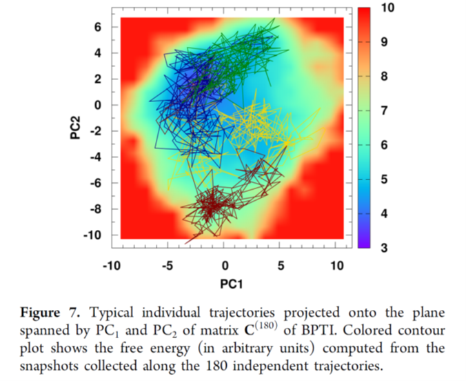
J. Chem. Inf. Mod., 57, 826-834 (2017)

data <- rnorm(1E5*100)
dim(data) <- c(1E5,100)
system.time(prcomp_data <- prcomp(data))

##    user  system elapsed 
##    4.66    0.03    4.75

system.time(princomp_data <- princomp(data))

##    user  system elapsed 
##    3.70    0.02    3.86

library(microbenchmark)
library(compiler)

sim <- function(l) {
  c <- rep(0,l); hits <- 0
  pow2 <- function(x) { x2 <- sqrt( x[1]*x[1]+x[2]*x[2] ); return(x2) }
  for(i in 1:l){
             x = runif(2,-1,1)
     if( pow2(x) <=1 ){
                  hits <- hits + 1
        }
        dens <- hits/i; pi_partial = dens*4; c[i] = pi_partial
         }
   
   return(c)
}

sim.comp0 <- cmpfun(sim, options=list(optimize=0))
sim.comp1 <- cmpfun(sim, options=list(optimize=1))
sim.comp2 <- cmpfun(sim, options=list(optimize=2))
sim.comp3 <- cmpfun(sim, options=list(optimize=3))

size <- 100000
bench <- microbenchmark(sim(size), sim.comp0(size), sim.comp1(size), sim.comp2(size), 
                        sim.comp3(size))

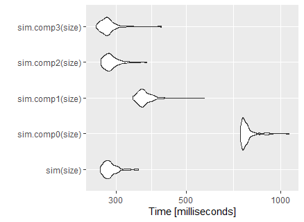
bench

## Unit: milliseconds
##             expr      min       lq     mean   median       uq      max neval
##        sim(size) 266.0428 277.2121 295.9702 291.1340 303.2662 497.4963   100
##  sim.comp0(size) 610.6016 630.1800 650.1550 638.5915 663.5033 784.7167   100
##  sim.comp1(size) 353.0935 375.8934 388.5088 382.2310 392.9938 617.0884   100
##  sim.comp2(size) 260.9811 279.4263 300.0358 291.8539 301.0266 515.4702   100
##  sim.comp3(size) 259.1039 280.2206 300.5654 291.1692 301.6518 474.2094   100

visualize the results:

library(ggplot2)
autoplot(bench)

Violin Plot

library(compiler)
enableJIT(level=3)

## [1] 3

bench <- microbenchmark(sim(size))
bench

## Unit: milliseconds
##       expr      min       lq     mean   median       uq      max neval
##  sim(size) 262.3286 273.5436 285.8035 287.4921 293.2419 412.3921   100

Rcpp package allows you to write your code in C++ that could be called within a R script:

library(Rcpp)

cppFunction('int mul(int a, int b, int c) {
  int mul = a * b * c;
  return mul;
}')
mul

## function (a, b, c) 
## .Call(<pointer: 0x0000000071281580>, a, b, c)

mul(2,4,6)

## [1] 48

Calling external functions (Fortran)

subroutine pifunc(n)
implicit none
integer, parameter :: seed = 86456
integer     :: i,n,hits
real        :: x,y,r,pival
call srand(seed)
hits = 0
do i=1,n
   x = rand()
   y = rand()
   r = sqrt(x*x + y*y)
   if(r <= 1) then 
       hits = hits + 1
   endif
enddo
pival = 4.0d0*hits/(1.0*n)
end subroutine pifunc

Calling external functions

One compiles the function using standard compilers (Linux, Kebnekaise):

gfortran -shared -fPIC -o picalc pi.f90

size <- 100000

dyn.load("picalc")
is.loaded("pifunc")
.Fortran("pifunc", n = as.integer(size))

Calling external functions

now we can benchmark our functions:

library(microbenchmark)
bench <- microbenchmark(sim(size), .Fortran("pifunc", n = as.integer(size)))
bench

#Unit: milliseconds
#                        expr        min         lq       mean     median         uq 
#          sim(size) 229.596323 234.312380 240.501156 236.034249 238.871773 316.289453
# .Fortran("pifunc")   4.136534   4.155587   4.239279   4.188102   4.261413   5.747752

Vectorized code performance was ~10 ms.

Calling Julia functions

ml GCC/8.2.0-2.31.1  OpenMPI/3.1.3; ml R/3.6.0; ml julia/1.1.0
library(JuliaCall) #install.packages("JuliaCall")
julia_setup()
julia_command("
function sim(l)
  hits = 0
  for i = 1:l
    x = rand()*2 - 1
    y = rand()*2 - 1
    r = x*x + y*y
    if r < 1.0 
      hits += 1
    end
  end
  pi_partial = (hits/l)*4
end")
invisible(julia_call("sim", size))

Calling Julia functions

library(microbenchmark)
bench <- microbenchmark(sim(size), julia_call("sim", size))
bench

#Unit: microseconds
#                    expr        min         lq        mean     median         uq  
#               sim(size) 230284.183 237486.927 246621.8263 244825.215 250872.803
# julia_call("sim", size)    400.051    426.745    490.8316    496.087    542.283

• Profile/benchmark your initial code to have a baseline

• Some techniques that can help you to get a faster code are

  • vectorization
  • pre-allocating objects
  • use matrices instead of Data Frames (Data Tables?)
  • check different functions/package implementations
  • use byte compiled code
  • if extra improvement is needed, it is time to consider Rccp or external function calls
  • calling Julia functions can also be helpful

• R High Performance Programming. Aloysius, Lim; William, Tjhi. Packt Publishing, 2015.
• http://adv-r.had.co.nz/Profiling.html#vectorise
• http://adv-r.had.co.nz/Functionals.html#functionals
• Pi vectorization
• Advanced R, Hadley Wickham, Taylor & Francis Group

Return to Index