- summary of the times spent in different function calls
- memory usage report
Feb., 2021
Profiling
Pi calculation

\(\textrm{Surface circle} = \left ( \frac{\textrm{Surface circle}}{\textrm{Surface square}} \right ) * (\textrm{Surface square})\)
is always valid. Knowing that \(\textrm{Surface circle} = \pi * r^2\), \(\pi\) can be computed as:
\(\pi = \frac{1}{r^2} \left ( \frac{\textrm{Surface circle}}{\textrm{Surface square}} \right ) * (\textrm{Surface square})\)
the ratio in parentheses is approximated with a Monte Carlo process throwing random points
Pi calculation

Surface ratio
- The R function to compute Pi is: Pi function adapted from: https://www.r-bloggers.com/2012/10/estimation-of-the-number-pi-a-monte-carlo-simulation/
sim <- function(l) {
 c <- rep(0,l)
 hits <- 0
 pow2 <- function(x) {
   x2 <- sqrt( x[1]*x[1]+x[2]*x[2] )
   return(x2)
 }
 for(i in 1:l){
   x = runif(2,-1,1)
   if( pow2(x) <=1 ){
     hits <- hits + 1
   }
   dens <- hits/i
   pi_partial = dens*4
   c[i] = pi_partial
 }
 return(c) }
Pi calculation
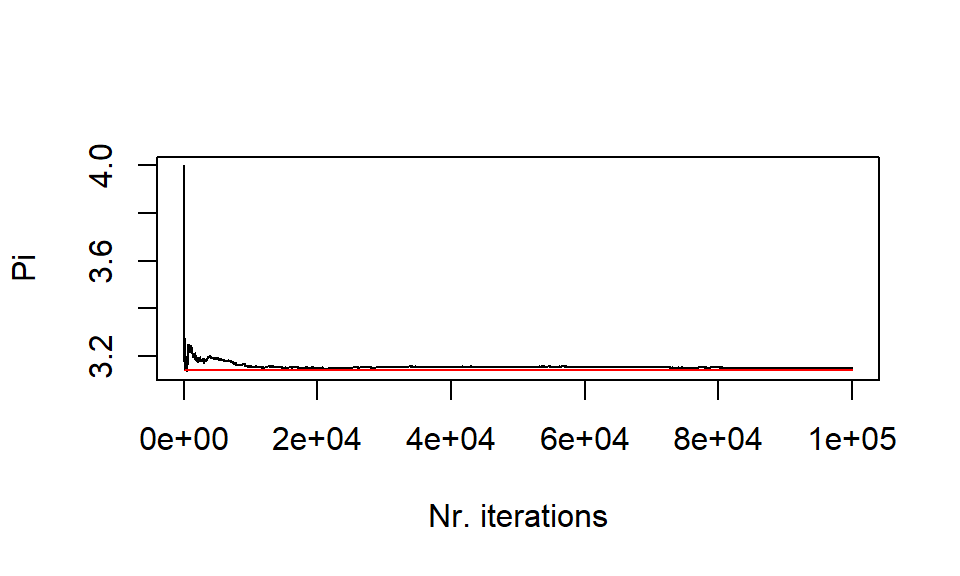
The accuracy of the calculation increases with the number of iterations
size <- 100000
res <- sim(size)
plot(res[1:size],type='l', xlab="Nr. iterations", ylab="Pi")
lines(rep(pi,size)[1:size], col = 'red')
Monitoring the execution time
System.time
This function is included in R by default
size <- 500000
system.time(
 res <- sim(size)
)
##    user  system elapsed
##    1.58    0.00    1.58
Monitoring the execution time
Tic toc
Another way to obtain execution times is by using the tictoc package:
install.packages("tictoc")
one can nest tic and toc calls and save the outputs to a log file:
Monitoring the execution time
Tic toc
library("tictoc")
size <- 1000000
sim2 <- function(l) {
   c <- rep(0,l)
   hits <- 0
   pow2 <- function(x) { x2 <- sqrt( x[1]*x[1]+x[2]*x[2] );  return(x2) }
   tic("only for-loop")
   for(i in 1:l){
      x = runif(2,-1,1)
      if( pow2(x) <=1 ){ hits <- hits + 1 }
      dens <- hits/i; pi_partial = dens*4; c[i] = pi_partial
   }
   toc(log = TRUE)
   return(c)
}
Monitoring the execution time
Tic toc
tic("Total execution time")
    res <- sim2(size)
## only for-loop: 2.96 sec elapsed
toc(log = TRUE)
## Total execution time: 2.97 sec elapsed
Monitoring the execution time
Tic toc
tic.log()
## [[1]]
## [1] "only for-loop: 2.96 sec elapsed"
##
## [[2]]
## [1] "Total execution time: 2.97 sec elapsed"
tic.clearlog()
Rprof
Rprof should be present in your R installation. For a graphical analysis, we will use proftools package. One needs to install this package in case it is not already installed. For R versions < 3.5 the instructions are:
install.packages("proftools")
source("http://bioconductor.org/biocLite.R")
biocLite(c("graph","Rgraphviz"))
while for R > 3.5 one needs to do
install.packages("proftools")
if (!requireNamespace("BiocManager", quietly = TRUE))
  install.packages("BiocManager")
BiocManager::install()
BiocManager::install(c("graph","Rgraphviz"))
Rprof
the profiling is performed with the following lines:
size <- 500000
Rprof("Rprof.out")
res <- sim(size)
Rprof(NULL)
Rprof
the profiling is performed with the following lines:
summaryRprof("Rprof.out")
## $by.self
##         self.time self.pct total.time total.pct
## "runif"      0.82    51.25       0.82     51.25
## "sim"        0.56    35.00       1.60    100.00
## "pow2"       0.22    13.75       0.22     13.75
##
## $by.total
##                          total.time total.pct self.time self.pct
## "sim"                          1.60    100.00      0.56    35.00
## "block_exec"                   1.60    100.00      0.00     0.00
## "call_block"                   1.60    100.00      0.00     0.00
## "eval"                         1.60    100.00      0.00     0.00
## "evaluate"                     1.60    100.00      0.00     0.00
## "evaluate::evaluate"           1.60    100.00      0.00     0.00
## "evaluate_call"                1.60    100.00      0.00     0.00
## "FUN"                          1.60    100.00      0.00     0.00
## "generator$render"             1.60    100.00      0.00     0.00
## "handle"                       1.60    100.00      0.00     0.00
## "in_dir"                       1.60    100.00      0.00     0.00
## "knitr::knit"                  1.60    100.00      0.00     0.00
## "lapply"                       1.60    100.00      0.00     0.00
## "process_file"                 1.60    100.00      0.00     0.00
## "process_group"                1.60    100.00      0.00     0.00
## "process_group.block"          1.60    100.00      0.00     0.00
## "render"                       1.60    100.00      0.00     0.00
## "render_one"                   1.60    100.00      0.00     0.00
## "rmarkdown::render"            1.60    100.00      0.00     0.00
## "rmarkdown::render_site"       1.60    100.00      0.00     0.00
## "sapply"                       1.60    100.00      0.00     0.00
## "suppressMessages"             1.60    100.00      0.00     0.00
## "timing_fn"                    1.60    100.00      0.00     0.00
## "withCallingHandlers"          1.60    100.00      0.00     0.00
## "withVisible"                  1.60    100.00      0.00     0.00
## "runif"                        0.82     51.25      0.82    51.25
## "pow2"                         0.22     13.75      0.22    13.75
##
## $sample.interval
## [1] 0.02
##
## $sampling.time
## [1] 1.6
Rprof
here you can see that the functions runif and pow2 are the most expensive parts in our code. A graphical output can be obtained through the proftools package:
library(proftools)
p <- readProfileData(filename = "Rprof.out")
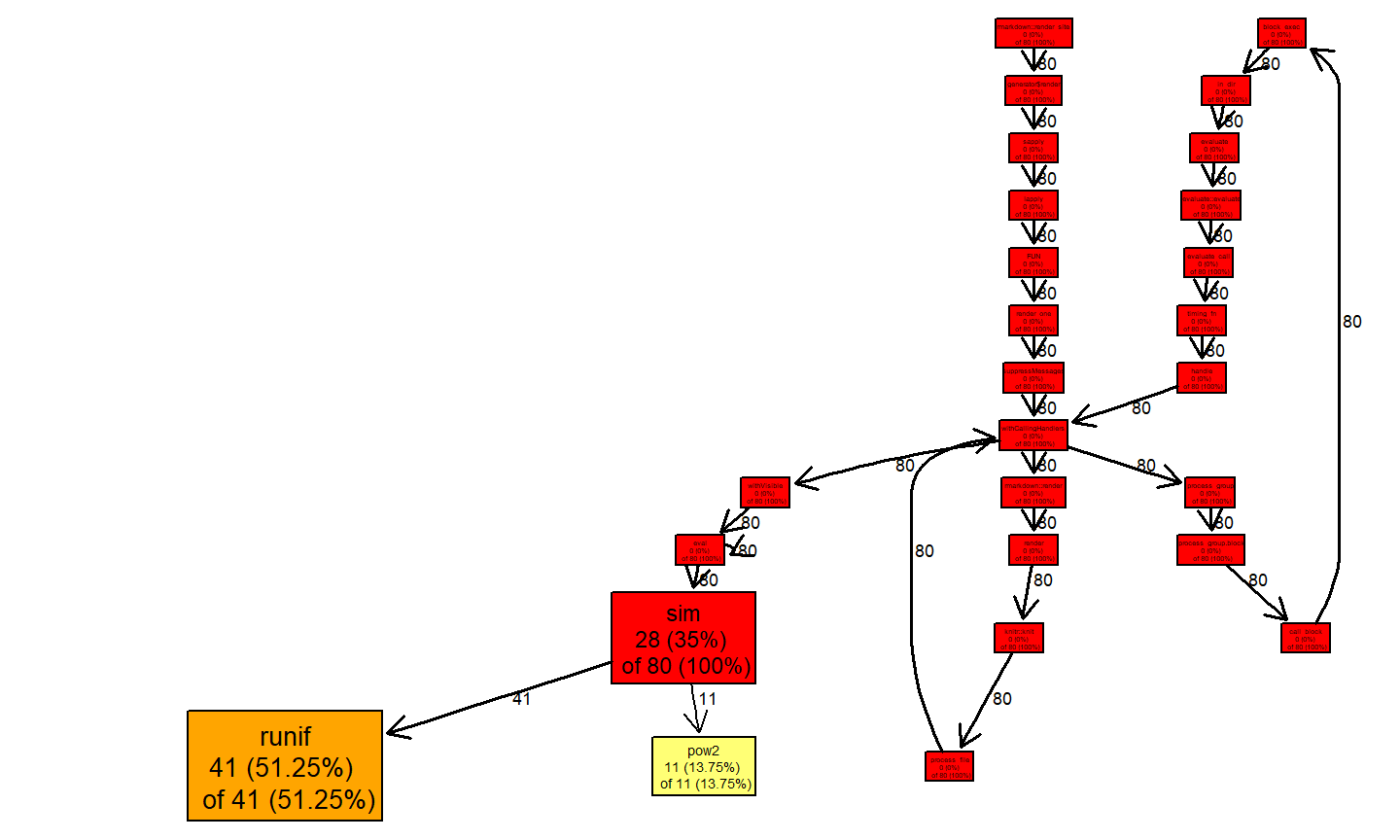
Rprof
plotProfileCallGraph(p, style=google.style, score="total")
Rbenchmark
One most probably needs to install this package as it is not included by default in R installations:
install.packages("rbenchmark")
then we can benchmark our function sim()
library(rbenchmark)
size <- 500000
bench <- benchmark(sim(size), replications=10)
Rbenchmark
bench
##        test replications elapsed relative user.self sys.self user.child sys.child
## 1 sim(size)           10   15.03        1     14.97        0         NA        NA
the elapsed time is an average over the 10 replications we especified in the benchmark function.
Microbenchmark
If this package is not installed, do as usual:
install.packages("microbenchmark")
and do the benchmarking with:
library(microbenchmark)
bench2 <- microbenchmark(sim(size), times=10)
Microbenchmark
bench2
## Unit: seconds
##       expr      min       lq     mean  median       uq      max neval
##  sim(size) 1.437368 1.448631 1.493887 1.45538 1.488293 1.788415    10
in this case we obtain more statistics of the benchmarking process like the mean, min, max, …
Summary
Timing your R code is useful to see what parts require optimization or a better package.
system.time and tic-toc will give you a single evaluation of the time taken by some R code
rbenchmark, microbenchmark functions will give statistics over independent replicas of the code
More useful information from profiling functions will be obtained if one uses functions to enclose independent tasks in your code (remember pow2, runif in the Pi calculation)
Once you know what are the bottlenecks of your code, working on a few of the most expensive ones could be more effective than working on many less significative functions
References
- https://swcarpentry.github.io/r-novice-inflammation/
- https://www.tutorialspoint.com/r/index.htm
- R High Performance Programming. Aloysius, Lim; William, Tjhi. Packt Publishing, 2015.
- https://www.r-bloggers.com/estimation-of-the-number-pi-a-monte-carlo-simulation/