Introduction to task-based parallelism
Objectives
A quick reference to parallel computation and HPC.
Understand the basics of task-based parallelism.
Understand the theoretical benefits of task-based parallelism.
Parallel computation and HPC
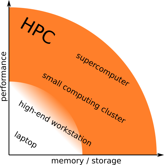
What is High Performance Computing?
High Performance Computing most generally refers to the practice of aggregating computing power in a way that delivers much higher performance than one could get out of a typical desktop computer or workstation in order to solve large problems in science, engineering, or business. (insideHPC.com)
- What does this mean?
- Aggregating computing power
Kebnekaise: 602 nodes in 15 racks totalling 19288 cores
Your laptop: 4 cores
- Higher performance
Kebnekaise: 728,000 billion arithmetical operations per second
Your laptop: 200 billion arithmetical operations per second
- Solve large problems
Time: The time required to form a solution to the problem is very long.
Memory: The solution of the problem requires a lot of memory and/or storage.
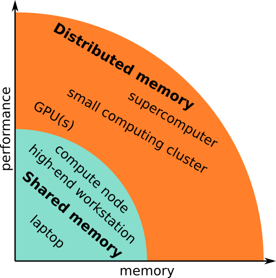
Memory models
When it comes to the memory layout, (super)computers can be divided into two primary categories:
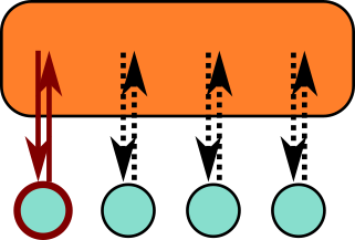
- Shared memory
A single memory space for all data:
Everyone can access the same data.
Straightforward to use.
- Distributed memory
Multiple distinct memory spaces for the data:
Everyone has direct access only to the local data.
Requires communication and data transfers.
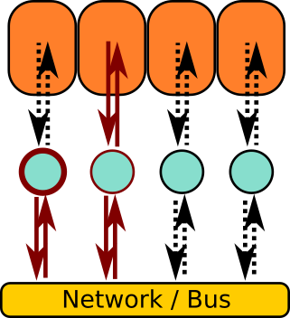
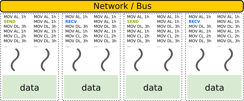
Computing clusters and supercomputers are generally distributed memory machines:
Programming models
The programming model changes when we aim for extra performance and/or memory:
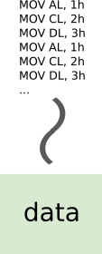
- Single-core
Matlab, Python, C, Fortran, …
Single stream of operations (thread).
Single pool of data.
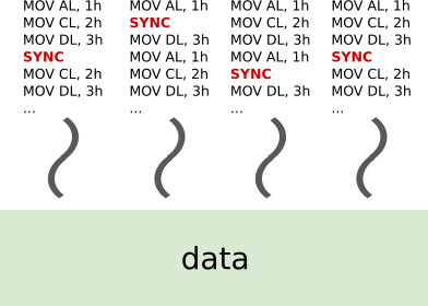
- Multi-core
Vectorized Matlab, pthreads, OpenMP
Multiple streams of operations (multiple threads).
Single pool of data.
Extra challenges:
Work distribution.
Coordination (synchronization, etc).
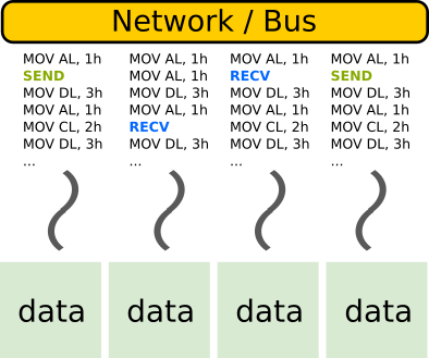
- Distributed memory
MPI, …
Multiple streams of operations (multiple threads).
Multiple pools of data.
Extra challenges:
Work distribution.
Coordination (synchronization, etc).
Data distribution.
Communication and data transfers.
- Accelerators / GPUs
CUDA, OpenCL, OpenACC, OpenMP, …
Single/multiple streams of operations on the host device.
Many lightweight streams of operations on the accelerator.
Multiple pools of data on multiple layers.
Extra challenges:
Work distribution.
Coordination (synchronization, etc).
Data distribution across multiple memory spaces.
Communication and data transfers.
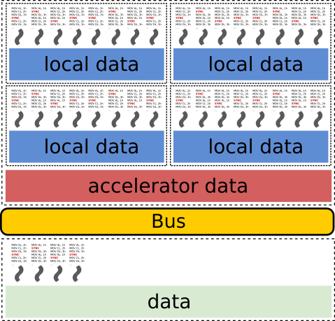
- Hybrid
MPI + OpenMP, OpenMP + CUDA, MPI + CUDA, …
Combines the benefits and the downsides of several programming models.
- Task-based
OpenMP tasks, StarPU
Does task-based programming count as a separate programming model?
StarPU = (implicit) MPI + (implicit) pthreads + CUDA
Functions and data dependencies
Imagine the following computer program:
1 2 3 4 5 6 7 8 9 10 11 12 13 14 15 16 | #include <stdio.h>
void function1(int a, int b) {
printf("The sum is %d.\n", a + b);
}
void function2(int b) {
printf("The sum is %d.\n", 10 + b);
}
int main() {
int a = 10, b = 7;
function1(a, b);
function2(b);
return 0;
}
|
The program consists of two functions, function1 and function2, that are called one after another from the main function.
The first function reads the variables a and b, and the second function reads the variable b:
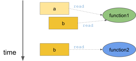
The program prints the line The sum is 17. twice.
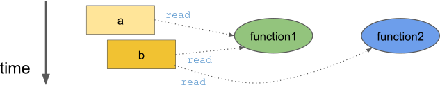
The key observation is that the two functions calls are independent of each other.
More importantly, the two functions can be executed in parallel:
Let us modify the the program slightly:
1 2 3 4 5 6 7 8 9 10 11 12 13 14 15 16 17 | #include <stdio.h>
void function1(int a, int *b) {
printf("The sum is %d.\n", a + *b);
*b += 3;
}
void function2(int b) {
printf("The sum is %d.\n", 10 + b);
}
int main() {
int a = 10, b = 7;
function1(a, &b);
function2(b);
return 0;
}
|
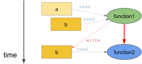
This time the function function1 modifies the variable b:
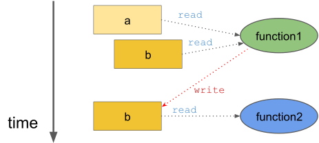
Therefore, the two function calls are not independent of each other and changing the order would change the printed lines. Furthermore, executing the two functions in parallel would lead to an undefined result as the execution order would be arbitrary.
We could say that in this particular context, the function function2 is dependent on the function function1.
That is, the function function1 must be executed completely before the function function2 can be executed:
However, this data dependency exists only when these two functions are called in this particular sequence using these particular arguments. In a different context, this particular data dependency does not exists. We can therefore conclude that the data dependencies are separate from the functions definitions.
Tasks and task dependencies
Based on the previous discussion, we need an object that can be described as the following:
The operation that is to be performed (implementation).
The data that is involved in the operation (input and output).
The way in which the operations are related to other operations (dependencies).
We call these objects tasks. The previous example code can be described using two tasks:
- Task 1
Operation:
function1.Input: variables
aandb.Output: updated variable
b.Depends on: none
- Task 2
Operation:
function2.Input: variable
b.Output: none.
Depends on: Task 1
We can represent the task dependencies using a Directed Acyclic Graph (DAG). This DAG is generally referred to as the task graph:
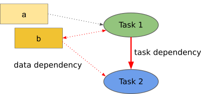
If we know what the sequential order to execute the tasks is, then we can deduce the task dependencies from the data dependencies. This is indeed what happens in practice as a programmer generally defines only
the task implementations, and
the input and output variables.
So-called runtime systems then deduce the task dependencies from the sequential order and the input and output variables. We say that the task graph is constructed implicitly. The runtime system then executes the task in a sequentially consistent order. That is, the runtime system may execute the task in any order as long as it respects the task dependencies.
A task-graph can also be constructed explicitly, i.e. a programmer defines both
the task implementations and
the task dependencies.
This can reduce the overhead that arises from the construction of the task graph.
More about task graphs
Let us consider a slightly more complicated situation. Consider an algorithm that consists of three steps that are iterated multiple times:
Compute a diagonal block (orange).
Update the corresponding block row and column (blue).
Update the corresponding trailing matrix (green).
We do not need to know how the tasks are implemented. We are only interested in the task dependencies:
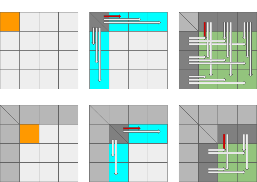
That is,
the block row and column updates are dependent on the computed diagonal block,
the trailing matrix updates are dependent on the block row and column updates, and
the next diagonal block is dependent on one of the trailing matrix updates.
Real-world task graph
We can represent these tasks and the related task dependencies using a task graph:
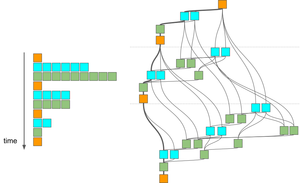
We can see that this task graph is much more complicated than the previous one. On the left, we can see how much parallelism can be exposed if we implement the algorithm using nested loops without considering the task graph:
for i = 1, ..., m:
    compute diagonal block A[i][i]
    parallel for j = i+1, ..., m:
        update block A[i][j] using A[i][i]
    parallel for j = i+1, ..., m:
        update block A[j][i] using A[i][i]
    parallel for ii = i+1, ..., m and jj = i+1, ..., m:
        update block A[ii][jj] using A[i][jj] and A[ii][i]
We can observe that the degree of parallelism decreases as the algorithm progresses. This can cause load balancing issues as more and more CPU cores become idle during the last iterations:
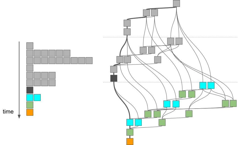
However, as shown on the right, we could have advanced to the same diagonal block by executing only a subset of the tasks. The delayed tasks can be used to keep the otherwise idle CPU cores busy.
Critical path
In this particular example, we have executed the tasks in such a manner that only the absolutely necessary tasks are executed. We can also find the longest path through the task graph (when measured in the terms of execution time):
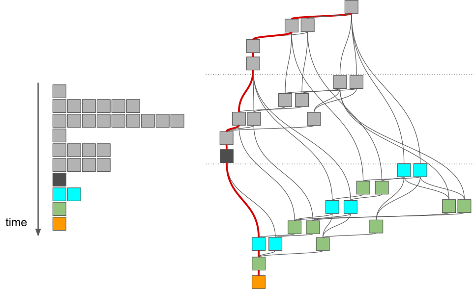
This so-called critical path gives us a lower bound for the execution time of the algorithm. The algorithm cannot be executed any faster than this no matter how many CPU cores are used. We can take advantage of the critical path only when we consider the task graph.
Task scheduling and priorities
Let us consider a different algorithm. Again, the details are not important as we only care about the data dependencies:
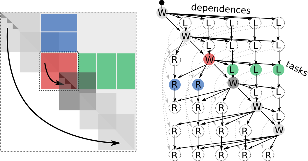
We can see that the task graph consists of three types of tasks:
- Process window (W)
Perform a computation operation inside a diagonal window (a set of small orthogonal transformations). In the above illustration, we have six overlapping diagonal windows.
- Right update (R)
Updates the matrix from the right (orthogonal transformation). Each process window task induces a set of right update tasks.
- Left update (L)
Updates the matrix from the left (orthogonal transformation). Each process window task induces a set of left update tasks.
We know two additional things about the algorithm:
The process window tasks are more time consuming than the left and right update tasks.
The left and right update tasks are equally time consuming.
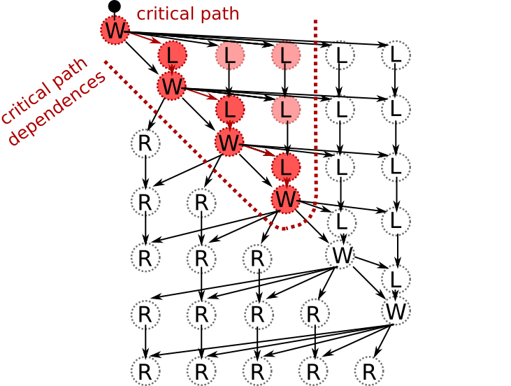
How should we schedule this task graph?
We can quite easily discover the critical path:
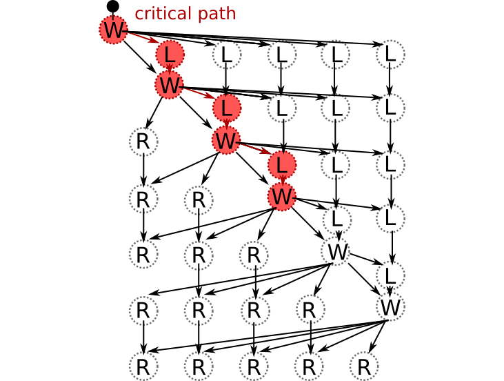
In order for us to advance along the critical path, we must also execute the critical path dependencies:
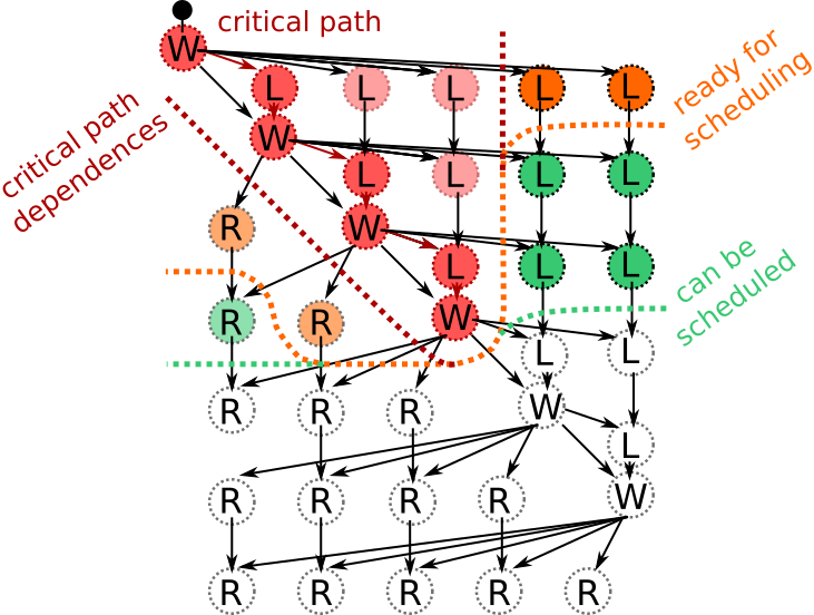
In the above illustration, we have executed only the critical path and its dependencies. However, we do not have to restrict ourselves in this manner since other tasks are ready for scheduling:
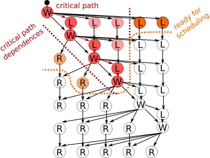
We could therefore use any idle cores to execute these tasks. However, since the left update tasks (L) feed back to the critical path, we may want to prioritize them over the right update tasks (R). This would indirectly accelerate the critical path as the next batch of left update tasks (L) becomes available earlier:
We must of course remember that task graphs are usually much more complicated than this:
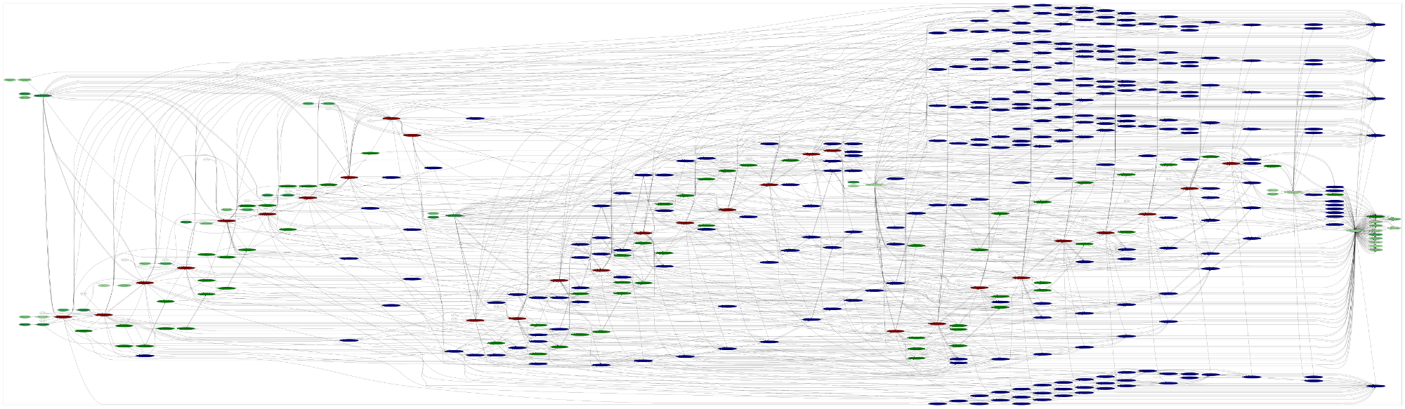
The above task graph comes from the so-called QR algorithm when it is applied to a very small matrix. We could probably figure out a close-to-optimal scheduling order from this task graph. However, the task graph is heavily preprocessed and its generation took several minutes whereas the execution time of the algorithm is just a few hundred milliseconds.
Heuristics scheduling approach
We therefore need an automated approach for traversing the task graph.
We have two options:
Analyse the entire task graph and locate the critical path. Schedule tasks that are on the critical path and their dependencies as early as possible.
Rely on heuristics.
The first approach would lead to optimal performance but assumes that
we know the entire task graph and
we know how long each task is going to take to execute.
We generally do not have this information, especially if we are dealing with an iterative algorithm.
Most runtime systems therefore rely on list-based heuristics and priorities. That is, a runtime system maintains four task pools:
- Submitted tasks
Tasks that are not scheduled and are not ready for scheduling.
- Ready tasks
Tasks that are not scheduled and are ready for scheduling.
- Active tasks
Tasks that are scheduled, i.e. are currently being executed.
- Completed tasks
Tasks that have been scheduled.
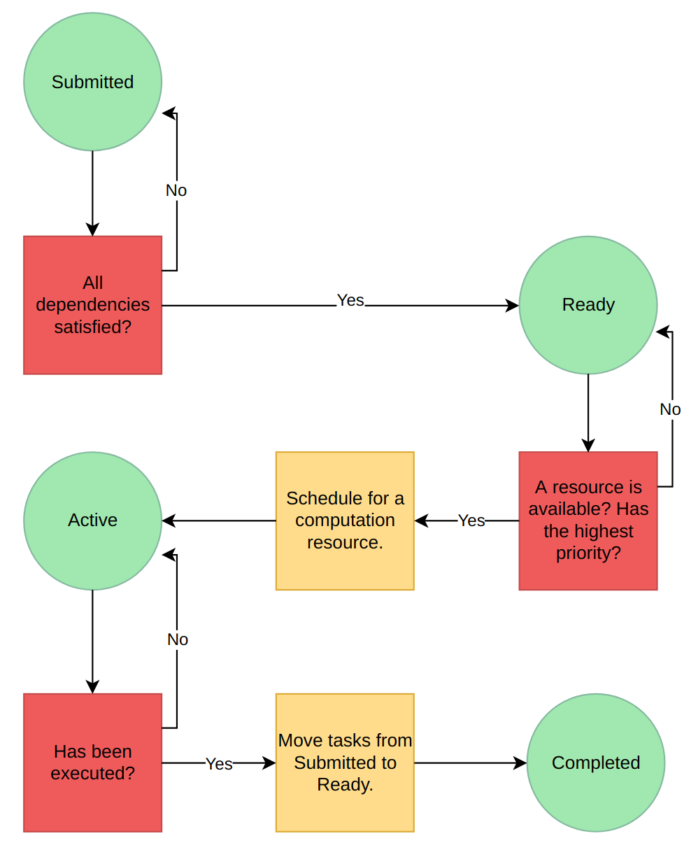
A runtime system follows these basic rules:
When a task becomes ready for scheduling, i.e. all its dependencies have been satisfied, it is moved from the submitted pool to the ready pool.
A task is moved from the ready pool to the active pool when it is scheduled for execution on a computational resource.
A programmer may define a priority for each task. These priorities are taken into account when a task is selected for execution from the ready pool.
A task is moved from the active pool to the completed pool when the related computational resource has finished executing the task.
Any tasks, that depend on the current tasks and have all their other dependencies satisfied, are moved from the submitted pool to the ready pool.
This approach is relatively simple to implement using (ordered) lists. However, the runtime system’s view of the task graph is very narrow as it sees only the ready pool when it is doing the actual scheduling decisions. In particular, note that the task priorities take effect only when a task becomes ready for scheduling.
Task granularity
Task granularity tells us how “large” the tasks are and how many of them there are. This can affect the performance because
the use of the runtime system introduces some additional overhead,
different task sizes lead to different task-specific performance, and
the ready pool size depends on the initial submitted pool size.
For example, consider the earlier example:
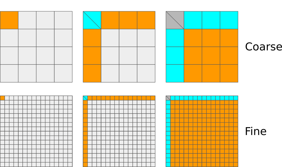
If the task granularity is very coarse, then
the number of tasks is very low and the runtime system therefore does not introduce that much overhead,
the tasks are relatively large and have a relatively high task-specific performance, and
only a very small number of tasks can be ready for scheduling at any given time.
If the task granularity is very fine, then
the number of tasks is very high and the runtime system therefore introduces a lot of additional overhead,
the tasks are very small and have a very low task-specific performance, and
a very large number of tasks can be ready for scheduling at any given time.
It is therefore very important that the task granularity is balanced:
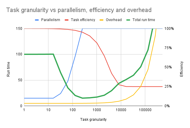
Both of these extremes lead to lowered performance. We want to keep most computational resources busy most of the time.
Benefits of task-based parallelism
Let us summarise some of the major benefits of task-based parallelism:
- Automatic parallelism
If the task task graph has potential for parallel computation, then the runtime system can discover it. An algorithm that has been implemented in a task-manner can therefore parallelise automatically.
- No synchronization
A parallel algorithm often involves several synchronization points. Sometimes these synchronization points arise from the underlying data dependencies. However, it is quite often the case that synchronisation points are used to simplify the implementation. The latter type of synchronisation points are not necessary in a task-based implementation.
- Better load balancing
The tasks are scheduled dynamically to the various computational resources. Furthermore, low-priority tasks can be delayed until the computational resources start becoming idle. These two factors help to improve the load balancing.
- Shortened critical path
If we help the runtime system by defining priorities, the runtime system can complete the critical path earlier.
- GPUs and other accelerators
Tasks can be scheduled to accelerator devices such as GPUs. This can happen dynamically using performance models (StarPU).
- Distributed memory
The task graph and data distribution induces the necessary communication patterns (StarPU).